
[ad_1]
Understanding past climate change is essential for putting modern global warming in context. Climate reconstructions during the Holocene – the current interglacial epoch, which began 11,700 years ago – based on geological evidence suggest that a peak in global average annual temperatures between 10,000 and 6,000 years was followed. a cooling trend, which was then reversed in the post-industrial era1,2. However, computer simulations of the Holocene climate reveal only a long-term warming trend.3. Write in Nature, Bova et al.4 report an analysis that effectively brings Holocene climate reconstructions in line with computer simulations. This result has important implications for our understanding of the drivers of climate change during the Holocene and for the context of post-industrial warming.
To reconstruct past climates, scientists rely on proxies: geological materials whose properties can be measured and correlated with modern climatic parameters. The apparent temperature peak in the early Holocene (known as the Holocene thermal maximum) is an important feature in global syntheses of proxy-based climate reconstructions.1,2 (Fig. 1). Its notable absence in computer modeling has been dubbed the Holocene temperature conundrum and has puzzled climatologists for years.3. The disagreement has been attributed to seasonal biases in the proxy reconstructions5 – that is, the approximations reflect changes in seasonal temperatures, rather than mean annual temperatures – and gaps in modeling6. Notably, global approximation syntheses are dominated by sea surface temperature (SST) recordings (see ref. 2, for example)2, which are known to have a seasonal bias5.
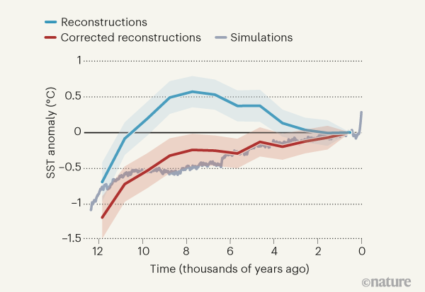
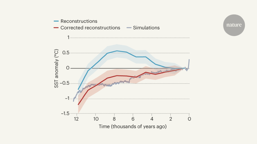
Figure 1 | Correction of seasonal biases in climatic reconstructions. Average global temperatures during the Holocene (the current interglacial epoch, which began 11,700 years ago) can be reconstructed from geological data. These reconstructions (blue line) suggest that sea surface temperatures (SST) peaked 10,000-6,000 years ago and then declined until the post-industrial period, when temperatures began to rise. However, computer simulations of Holocene SST do not match these reconstructions, possibly because the geological records are seasonally biased – the records reflect changing seasonal temperatures rather than mean annual temperatures. Bova et al.4 report a method that quantifies and corrects for seasonal biases in marine geological records, and use it to estimate mean annual SST (red line). The corrected data correspond to computer simulations, thus solving a long-standing problem in this area. The SST are represented as anomalies: the difference between the SST of a reference time interval and the average SST between 0 and 1000 years. Shaded areas represent the limits of a standard error.
The new method by Bova and colleagues identifies seasonal biases in SST records and allows the calculation of the mean annual SST from the seasonal SST. It takes advantage of the characteristics of the last interglacial period (128,000 to 115,000 years ago), which was marked by mild global temperatures, smaller ice caps and higher sea levels than today. ‘hui.seven. This period is advantageous for the purposes of the authors in that the seasonal difference in incoming solar radiation (insolation) was greater than during the Holocene, while the effects of other climate-modifying factors, such as greenhouse gases greenhouse and ice, were weaker, making it easier to identify seasonal biases.
Specifically, the authors’ method consists of identifying the seasonal bias in the part of an SST record that corresponds to the last interglacial, and in which there was a stronger correlation of SST with seasonal insolation than with average annual insolation. The sensitivity of the SST recording to seasonal insolation during this period is then calculated and used as a reference point to remove the seasonal bias from the entire recording, thus allowing the average annual SST to be determined from this. recording. The authors first applied their method to a proxy-based SST reconstruction taken from a marine site off the northeast coast of Papua New Guinea. The transformed average annual SST record was independently validated by applying the new method to the SST data for the same geographic region produced in the computer simulations of the last 300,000 years – the transformed data corresponded to the average annual SST output of the simulations.
Bova et al. then created a synthesis of previously published SST records covering the latest interglacial and Holocene periods. These records are based on two common proxies used to reconstruct SST: the chemical composition of the fossilized calcium carbonate shells of unicellular marine organisms living on the surface called foraminifera; and organic biomarkers called alkenones, which are synthesized by marine algae and are deposited in marine sediments. The authors found that the majority of SST records examined are indeed seasonally biased.
After converting the seasonally biased SST records to average annual SST records, Bova and his colleagues deduce that the climate has been warming since the start of the Holocene – that is, there is no evidence of ‘a Holocene thermal maximum in mean annual temperatures (Fig. 1). Rather, they suggest that the Holocene thermal maximum is a seasonal feature driven by a peak summer insolation in the northern hemisphere that occurred at the start of the Holocene.
The reconstruction of the mean annual temperatures produced from the synthesis by the authors of proxy records strongly resembles a computer simulation3 of the Holocene climate which also reflects mean annual temperatures – effectively solving the Holocene temperature conundrum. This allowed Bova and his colleagues to shed new light on the drivers of Holocene climate change. They find that the increase in global average annual temperatures that occurred during the early Holocene (12,000 to 6,500 years ago) was a response to the retreat of the ice caps, while the continued increase in temperatures over the 6 Past 500 years is due to increasing concentrations of greenhouse gases. .
The authors also show that the mean annual temperatures during the last interglacial period were more stable and higher than their estimates of Holocene temperatures. They attribute this to the near constant concentrations of greenhouse gases and the reduction in the extent of the ice caps during the last interglacial. Importantly, the researchers find that the current mean annual temperature exceeds those of the past 12,000 years and is probably approaching the heat of the last interglacial period.
Bova and colleagues’ method for identifying and correcting seasonal biases in proxy SST reconstructions can now be applied to other temperature recordings at different time scales. This is a key benefit of their study, because paleoclimatic scientists have long known that temperature reconstructions are likely seasonally biased, but lacked a method to solve the problem.
One limitation of the results is that the new synthesis of proxy SST records is limited to the global region between 40 ° N and 40 ° S. Proxy records from higher latitudes have been deliberately excluded due to the scarcity of these records for the latter. interglacial, and because of the proximity of these regions to ocean fronts, where ocean dynamics can affect SST. However, the inclusion of these regions may be necessary in the future, as the processes at high latitudes play a substantial role in many climate feedback processes. Additionally, the new summary examines records based on only two SST proxies. Future work should include more recordings based on other temperature indicators. Nonetheless, by solving a conundrum that has baffled climatologists for years, the study by Bova and his colleagues is a major breakthrough for the field.
[ad_2]
Source link